Graphs are a powerful way to model relationships between objects, and representing them effectively is crucial for many algorithms in computer science and network analysis. One of the most commonly used representations for graphs is the Adjacency Matrix. In this blog post, we’ll explore what an adjacency matrix is, how it works, and its applications with examples.
What is an Adjacency Matrix?
An Adjacency Matrix is a 2D array (or matrix) used to represent a graph. It’s a square matrix where the rows and columns correspond to vertices of the graph, and the entries in the matrix represent the presence (and possibly the weight) of edges between vertices.
Structure of an Adjacency Matrix
- Size: For a graph with ( n ) vertices, the adjacency matrix is an ( n \times n ) matrix.
- Entries: The entry ( A[i][j] ) indicates whether there is an edge from vertex ( i ) to vertex ( j ).
- Unweighted Graphs: In unweighted graphs, ( A[i][j] ) is
1if there is an edge from vertex ( i ) to vertex ( j), and0otherwise. - Weighted Graphs: In weighted graphs, ( A[i][j] ) contains the weight of the edge between vertices ( i ) and ( j), and
0(or∞) if no edge exists.
Example of an Adjacency Matrix
Consider this simple graph:
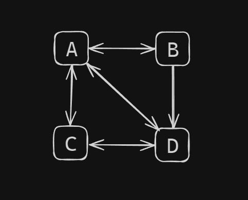
The adjacency matrix for this unweighted graph would be:
   A B C D
A  0 1 1 1
B  1 0 0 1
C  1 0 0 1
D  1 1 1 0
Explanation:
- ( A[0][1] ) and ( A[1][0] ) are
1because there is an edge between vertices A and B. - ( A[0][2] ) and ( A[2][0] ) are
1because there is an edge between vertices A and C. - ( A[0][3] ) and ( A[3][0] ) are
1because there is an edge between vertices A and D. - ( A[1][3] ) and ( A[3][1] ) are
1because there is an edge between vertices B and D. - ( A[2][3] ) and ( A[3][2] ) are
1because there is an edge between vertices C and D.
Adjacency Matrix for Directed Graphs
In directed graphs, the adjacency matrix reflects the direction of the edges. For example:
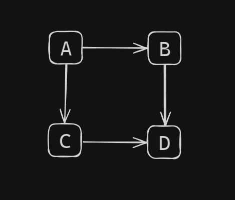
The adjacency matrix for this directed graph would be:
   A B C D
A  0 1 1 0
B  0 0 0 1
C  0 0 0 1
D  0 0 0 0
Explanation:
- ( A[0][1] ) is
1because there is a directed edge from A to B. - ( A[0][2] ) is
1because there is a directed edge from A to C. - ( A[1][3] ) is
1because there is a directed edge from B to D. - ( A[2][3] ) is
1because there is a directed edge from C to D.
Adjacency Matrix for Weighted Graphs
For weighted graphs, the adjacency matrix entries are the weights of the edges. Consider this weighted graph:
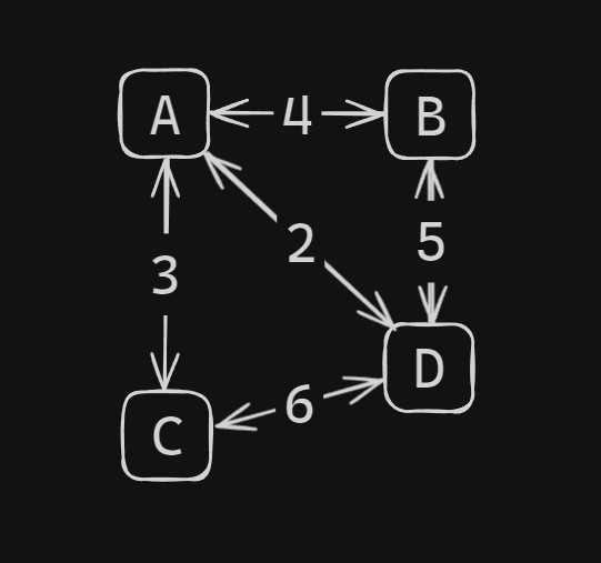
The adjacency matrix would be:
   A B C D
A  0 4 3 2
B  4 0 0 5
C  3 0 0 6
D  2 5 6 0
Explanation:
- ( A[0][1] ) and ( A[1][0] ) are
4because the edge between A and B has a weight of 4. - ( A[0][2] ) and ( A[2][0] ) are
3because the edge between A and C has a weight of 3. - ( A[0][3] ) and ( A[3][0] ) are
2because the edge between A and D has a weight of 2. - ( A[1][3] ) and ( A[3][1] ) are
5because the edge between B and D has a weight of 5. - ( A[2][3] ) and ( A[3][2] are
6because the edge between C and D has a weight of 6.
Advantages and Disadvantages of Adjacency Matrix
Advantages
- Simplicity: Adjacency matrices are straightforward to implement and understand.
- Fast Edge Lookup: Determining whether an edge exists between two vertices is O(1) time.
Disadvantages
- Space Complexity: Adjacency matrices require ( O(V^2) ) space, which can be inefficient for sparse graphs (graphs with relatively few edges compared to the number of vertices).
- Inefficient for Large Sparse Graphs: Storing and processing large sparse graphs can be memory-intensive and slow.
Applications of Adjacency Matrix
- Graph Algorithms: Many algorithms such as Floyd-Warshall for shortest paths and Prim’s algorithm for MSTs can be efficiently implemented using adjacency matrices.
- Network Analysis: Adjacency matrices are used in analyzing and visualizing network structures.
- Circuit Design: Used in representing and solving problems related to circuit design and analysis.
Java Implementation of Adjacency Matrix
Here’s a simple Java implementation to create and manipulate an adjacency matrix for an unweighted graph:
Java Code
import java.util.Scanner;

public class AdjacencyMatrix {
    private int[][] matrix;
    private int numVertices;

    public AdjacencyMatrix(int numVertices) {
        this.numVertices = numVertices;
        matrix = new int[numVertices][numVertices];
    }

    // Add edge
    public void addEdge(int src, int dest) {
        matrix[src][dest] = 1;
        matrix[dest][src] = 1; // For undirected graph
    }

    // Remove edge
    public void removeEdge(int src, int dest) {
        matrix[src][dest] = 0;
        matrix[dest][src] = 0; // For undirected graph
    }

    // Print the adjacency matrix
    public void printMatrix() {
        for (int i = 0; i < numVertices; i++) {
            for (int j = 0; j < numVertices; j++) {
                System.out.print(matrix[i][j] + " ");
            }
            System.out.println();
        }
    }

    public static void main(String[] args) {
        Scanner scanner = new Scanner(System.in);
        System.out.print("Enter number of vertices: ");
        int numVertices = scanner.nextInt();

        AdjacencyMatrix graph = new AdjacencyMatrix(numVertices);

        System.out.print("Enter number of edges: ");
        int numEdges = scanner.nextInt();

        for (int i = 0; i < numEdges; i++) {
            System.out.print("Enter edge (source and destination): ");
            int src = scanner.nextInt();
            int dest = scanner.nextInt();
            graph.addEdge(src, dest);
        }

        System.out.println("Adjacency Matrix:");
        graph.printMatrix();

        scanner.close();
    }
}
How the Code Works
- Initialization:
- Create an adjacency matrix of size ( numVertices \times numVertices ).
- Add Edge:
- The
addEdgemethod setsmatrix[src][dest]andmatrix[dest][src]to 1, indicating an undirected edge between verticessrcanddest.
- Remove Edge:
- The
removeEdgemethod setsmatrix[src][dest]andmatrix[dest][src]to 0, indicating the removal of the edge.
- Print Matrix:
- The
printMatrixmethod outputs the adjacency matrix to visualize the graph.
Example Output
If you input 4 vertices and 4 edges (0 1, 0 2, 1 3, 2 3), the output adjacency matrix would be:
Adjacency Matrix:
0 1 1 0
1 0 0 1
1 0 0 1
0 1 1 0
This represents the following graph:
0 -- 1
|    |
2 -- 3
Conclusion
The Adjacency Matrix is a fundamental tool in graph theory, offering a clear and efficient way to represent and work
with graphs. Its simplicity makes it a popular choice for small and dense graphs. However, for larger and sparse graphs, other representations like adjacency lists may be more appropriate. Understanding and using adjacency matrices effectively can greatly aid in solving complex problems related to networks, paths, and connectivity.
Feel free to experiment with the provided Java code and modify it to suit different types of graphs and applications. Happy coding!
This blog post should give beginners a solid understanding of what an adjacency matrix is, how it works, and how it can be implemented in Java. Let me know if you need more details or adjustments!